You’ll notice a lot of tables with regression in the name. This is a method of approximating output, assuming there is only 1 factor involved (I can’t figure out multi-variate linear regression yet), the defensive handicap. Below I will explain player average, defensive handicap and linear regression and how it is applied to make a better predictor of how a player will perform at his position, than just his average pts/game. So you understand the analysis in the database.
Fantasy football and sports gambling (and with more at stake, financial securities investment) has a some traits in common. Most of the people who play it, sell themselves as seers who can peer into the future about events. But investing is a lot like this as well, except the horses are companies. So business statistics can be used to analyze the player performances. So in this post, we will explain the application of statistics, to create a simple (but not terribly precise) prediction model to fantasy football production, is implemented in the database. First, the explanation of the data of the application.
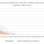
For the 2017 season, on a per game basis, all the players at every (pseudo)position that is scored by fantasy football averaged below, using 2 different scoring systems. Please take in mind, this is all the players, including the many many very marginal players.
| Scoring | Avg (pts) | St Dev |
| Standard | 3 | 5.651 |
| PPR | 7 | 7.314 |
But you need to keep in mind what reality is, and how theory of statistics has summarized the data to look like, with only 2 numbers to describe the entire dataset : average and standard deviation. Below shows what the theory predicts, vs actual numbers.
A real smart statistician will say, “you used the wrong model. There is no much thing as a typical player b/c they don’t all get same opportunity”, etc, etc. I’m not a real smart statistician, so I can’t tell you how I misapplied a normal distribution, to an event not centered around a single outcome value. However, it works rather well for a single player. And eventually, that’s where it is going to be used. I just need to show how theory and real life can differ.

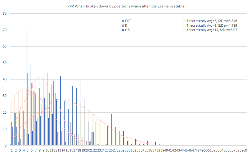
However, you can break it down by position, and notice that each position has distinct roles, which leads to their different levels of derivative production in the game of fantasy football. You’ll notice the implied points/gm ranges are different for every position. The points are produced from rules specifying the worth of each statistic, into points.
| Scoring | Pos | Avg (pts) | St Dev |
| PPR | DST | 5 | 5.846 |
| PPR | K | 8 | 4.789 |
| PPR | QB | 14 | 8.071 |
| PPR | RB | 7 | 7.587 |
| PPR | TE | 5 | 5.775 |
| PPR | WR | 7 | 7.222 |
| Standard | DST | 1 | 4.186 |
| Standard | K | 6 | 4.207 |
| Standard | QB | 8 | 7.976 |
| Standard | RB | 2 | 5.507 |
| Standard | TE | 4 | 3.750 |
| Standard | WR | 2 | 5.302 |
First thing you notice, is that players playing at some positions seem to “naturally” score more than others, indicated by the average. The other is that some positions offer more differentiation that others, indicated by larger standard deviation value. That differentiation has a lot of reasons, such as ability, opportunities, and competition. Indeterminate differentiation is bad for the purposes of creating reliable predictions. But differentiation is important in terms of draft strategy since each of your draft choices are opportunity costs to your competitors. The easiest way to think of it is, if the stdev is 0 for a position, it’s easy to predict, but every player scores exactly the same amount each week, so what is the difference between drafting one vs another, therefore why waste a early round draft pick? Here, we try to create a prediction model, to quantify the differentiation of each player compared to each other. Eventually, we use defense for a particular week on the schedule, to narrow the precision range for each week, hopefully better quantifying one player vs another for starting purposes, or future trade information. Quantifying here means making that range smaller where we are wrong about one player being better than the other. (ie. A player that averages 10 seems better than a player averaging 8, but is a player that scores between 6 to 14, better than a player scoring 0 to 16? Should you feel better or worse, if it was 7 to 9, compared to 6 to 14?)
Linear Regression’s R-number
has similar idea of smaller std dev, due to a correct prediction model. R is a measure of how much of the stdev of the sample, can be explained by the prediction model.
The first histogram (before) illustrates how the square peg of real game production was squeezed into theory’s curve. It doesn’t fit so well. But the x-range of the thicker parts of the blue curve, is also the x-range of the thicker parts of the red curve. So at least the range is useful, in that any prediction model we create, that produces a wider range of thickness than that first normal curve(before), then it is of no use. So our prediction model has to produce a smaller standard deviation. Below, we chart the individual game production for the positions of QB, K, and DST b/c they have somewhat pleasing normal curves b/c the roles usually belong exclusively to one person, so there aren’t a lot of players playing bit roles crowding the 1pt/gm space, as with WR, TE and RB. The opportunities/gm for the below charted positions are pretty much stable : 0pts and 1pt isn’t charted, or the entire game is monopolized by one pt players. The standard deviation of our prediction model ALSO HAS TO BE BETTER than the higher bar set by the lower standard deviation produced from using the position’s average.
Now to further expand the idea of standard deviation. One standard deviation (range between plus and minus the standard deviation from average) in statistics is generally thought to mean : 67% of the time, players will score in that range. So if you pick a random player, and a random game in past, and say you expect him to score in that game, inside the plus/minus range, you have a 67% chance of being right. But the past is the past…
What value is knowing the range where an occurrence is 67%? If you won $1 for being inside that range, and lost $1 for being outside that range, well you should make money. If those are the terms. Business statistics also call this a expected value (per occurrence). Future tense. $1*0.67 – $1*0.33 = 0.34. So if you bet 1000 times, you should have won on average $340, picking random games in past. There is a caveat. What happened in past isn’t the same in future. And the betting terms are never that good. You should pay attention to the position’s average, and the standard deviation and it’s implied range. In theory, any defense scores between -1 and 11 points in fantasy football, 67% of the time. That is a really wide range for a defense. Nothing special about picking a huge range of success. Who is going to offer you, a dollar inside that range and receive a dollar from you outside that range when you randomly select any game, on those terms, if they want to keep their money? More to the point of this post, if we were trying to create a prospectus on each player using this information, before we drafted him vs another player, the position average would offer next to no information on which is a better choice. But we at least establish the outer envelope of what is arguably considered reasonable prediction material. There is no less precise, but still rational way of predicting how a specific independent player will do in future, than to say that at the very least, the prediction model should be more precise than using the same number every week: the average of all player production.
So we try to narrow this prediction range. Below, we take the average for each player, and say what HE did in the past, is what he is going to do in the future. Below are the results of the standard deviation using the player’s average, compared to standard deviation to population sample, when we use a player’s average as the predictor of his performance for next week. There are also predictors that take the defense he faces as a handicap. And another predictor that assumes that different players are handicapped differently when faced with different quality defenses.
Is what a player does in the past, always what he will do in the future? No, obviously. In the real world, you wouldn’t risk your life on it, maybe your worst enemy, and then how many of our worst enemies actually deserve death. But the world of statistics say, if all the same conditions are true, he should score the same every week, and if he doesn’t, those are caused by sources of error we can’t measure and create a educated fudge factor for. Same factors like teammates, same field, same rules, same coach, average defense. The basis of our best guess.
| Scoring system | Method of determining Expected Value | Stdev using EV | Stdev of NFL avg |
| PPR | Season Running Average as Expected Value | 6.56998 | 7.31453 |
| PPR | Season Running Average as Expected Value, w/ defensive handicap to average | 2.35938 | 7.31453 |
| PPR | Season Running Average as Expected Value, linearly approximated by player defense coefficient | 5.74305 | 7.31453 |
| PPR | Trailing 17-Week Average as Expected Value | 6.60184 | 7.31453 |
| PPR | Trailing 17-Week Average as Expected Value, w/ defensive handicap to average | 3.23164 | 7.31453 |
| PPR | Trailing 17-Week Average as Expected Value, linearly approximated by player defense coefficient | 3.90026 | 7.31453 |
| Standard | Season Running Average as Expected Value | 5.65408 | 5.65188 |
| Standard | Season Running Average as Expected Value, w/ defensive handicap to average | 2.37438 | 5.65188 |
| Standard | Season Running Average as Expected Value, linearly approximated by player defense coefficient | 5.05318 | 5.65188 |
| Standard | Trailing 17-Week Average as Expected Value | 5.41071 | 5.65188 |
| Standard | Trailing 17-Week Average as Expected Value, w/ defensive handicap to average | 3.66088 | 5.65188 |
| Standard | Trailing 17-Week Average as Expected Value, linearly approximated by player defense coefficient | 3.60903 | 5.65188 |
Obviously, just by using the player’s own average to predict the next game, rather than the average NFL production of fantasy points, you can see a significant reduction in the standard deviation, and implied better precision. And there are 3 different methods of producing the expected value. Each accounts for an additional variable which we hypothesize affects fantasy point production.
The three methods are
- Using the player’s average, to use as the predicted value for next game
- Using the player’s average, subtract a handicap representing a good defense he faces (and vice versa), to use as the predicted value for next game
- Assume each player responds differently to a good or bad defense. This response is approximated by an equation pts=player average + defense*player coefficient.
Theoretically, each method should produce a better and better approximation.
When there isn’t enough data in a season, the moving 17-week average is used. Season data is best b/c the teammates should be the same, rules the same, and coach, etc. Different seasons for a player, is like being on a different team. It’s better than nothing at all, but we want things we measure to have the same conditions, as the thing we are predicting, to rule out sources excuses why the prediction didn’t work.
Handicap is a simple calculation that takes every team that has faced another team. Takes the team’s total actual fantasy football point output during that game. And divides it by the team average for the season. The average of that average, is the handicap for a team. A good defense theoretically will cause most players to produce less output, and therefore lower the average. We are calculating lowered or heightened total aggregate output from an offensive position. Individual output can change drastically esp with the bit players who normally score 1 pt and get 5 pts and it looks like a 500% increase, so then we have to weigh the average by their avg point output, so it doesn’t skew the results.
Example: Hypothetical Stats to quantify how a defense handicaps fantasy point production
WAS RB scored 4 against Pats/(8pts/gm) = 0.5
NYG RB scored 14 against Pats/(28pts/gm) = 0.5
SF RB scored 15 against Pats/(20pts/gm) = 0.75
…
MIA RB scored 16 against Pats/(12pts/gm) = 1.333
———————————————
Avg is 0.85
This handicap factor is used in the two ways above. The first is simply multiplying the handicapping factor of the defense the player faces, to his average. We are basically saying we expect him to score less this much, b/c most players have in the past.
The third method, and 2nd method that uses the defense handicap, uses linear regression to find out how a player reacts to the defensive handicap factor. This referred to as the player coefficient (there are 2 coefficients, but one is usually the average, so the other is referred to as the player coefficient to the defense term). A coefficient of 1, is the same as previous method. But if they have a coefficient of 2, this means that the player does well against bad defenses, and absolutely horrible against good ones. A coefficient of 0.2 means the player probably assumes good defenses all the time, and doesn’t take the high risk high reward chances that work against a good defense, so he doesn’t falter that much against a good defense. But probably doesn’t do that well against a bad one either.
You obviously can start throwing in a whole bunch of other stuff like home/road splits. Weather. Coach. Players on line, etc. But I kept it to defense handicapping. Esp since SQL server doesn’t have a built-in aggregate function for linear regression, so I have to write several queries, for regression on one pair of data points.
But Excel does. Check my results if you like.
I’ll post the .MDB file for the SQL Server LocalDB, so you have run your own queries.